The goal of this project was to predict a Windows machine’s probability of getting infected by numerous types of malware, based on telemetry data provided by the user’s computer or mobile device, and threat reports generated by Microsoft’s built-in anti-malware solution, Windows Defender.
![]()
Each row of the data provided by Microsoft corresponds to a unique machine, identified by its MachineID in the data. The data contains 8,921,483 entries in the train.csv training set, and we must use this data to predict whether we will find malware on the 7,853,253 entries in the test.csv testing set, represented by the HasDetections field in the data.
Preparing the Data
Extracting Relevant Features
One of the biggest challenges that I encountered while working with this dataset was simply storing the whole dataset in memory! With almost 17 million rows in the training and testing set combined, I had to get creative with how to store it in the same instance. To combat this, I wrote a function that finds the smallest datatype holder possible for each column of the data and then set those datatypes from the beginning when importing data to save space from the get-go.
Once the data was in memory, I reduced the number of features provided in the data by only keeping columns with less than 50% missing values and columns where the most common value occurs less than 95% of the time. This filtering process reduced the data from 83 columns to 60 columns.
Cleaning and Wrangling Remaining Features
After the features that met these criteria were extracted, I needed to preprocess the data to make it easier to work with.
First, I split the data into numerical features, binary features, and categorical features to impute missing values accordingly.

For the numerical features and categorical features that are represented with numbers, I filled missing values with -1. For the binary features, I filled missing values with the most common value in the column. For the remaining features, I handled each of the columns by hand. To do this, I followed a general 4-step process:
- Convert values to lowercase.
- Merge values of different spellings.
- Set NA values to ‘unknown’.
- Merge or set uncommon values to ‘unknown’.
After processing the remainder of the features, they are now ready for numerical encoding, which allows the data to be fed into a machine learning model.
Encoding the Data
The binary and numerical features are already ready to feed into the model, so we need to encode the categorical features since the model can’t perform operations on text data. I decided to treat these features in one of two ways — label encoding (assigning each unique value in the column a different integer), or frequency coding (label encoding, but values are assigned in ascending order based on their frequency in the data).
Machine Learning Models
Baseline Models
Now that all the features are cleaned up and encoded as integers, the model is finally ready to work with the data. Training the models with all 17 million rows of the data and iterating different types of models would have taken too long given the timeframe of the project, so I opted to take a 5% random sample of the data and train my models with that, reducing the training to set to only ~450,000 rows.
From these 450,000 rows, I split them into 80% train and 20% validation sets to identify the basic performance of the models. I honestly didn’t spend too much time on iterating through different models to find the best performance, since I was running out of time to complete the project, but both models perform better than the baseline guess of 50% accuracy.
The first model I chose to test was a Random Forest classifier. The validation accuracy for this model was 62.73%. The second model I chose was Logistic Regression, which had a slightly lower accuracy of 60.11%. Since the Random Forest had a higher validation accuracy, I used this model for the prediction on the whole test set.
Using only 5% of the training data available, I was able to reach a test accuracy of 59.22% with default hyperparameters. While this score is far from the best (top scorers in this challenge reached a test accuracy of at least 69.8%). For tasks like these, more complicated tree-based models like XGBoost might be preferred and provide a higher test accuracy, but I will explore that when improving on this work in the future.
Model Explanations
I chose two visualizations to help explain the choices of the Random Forest.

The first visualization is an ELI5 feature importance chart that shows each feature’s weight contributed to the decision in the Random Forest. A higher weight indicates that the feature is more important to the overall performance of the model and should be given higher priority.
As you can see, some of the features have a zero or even negative weight, indicating that the model would perform the same or better by omitting those features in the final model.
Ideally, those would be eliminated before processing the data, since it would save space and computation time in the long run. This figure does not include all of the features used in the final model, particularly those with negative scores, but we can see that their inclusion is unnecessary.
The second visualization is a SHAP (SHapley Additive exPlanations) explanation force plot for the first entry in the test set.
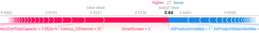
Using the SHAP explanation force plot, we can see the features that contributed most to the model’s predicted probability for each entry in the data. Here, we see that SmartScreen = 3 gives the highest positive effect and AVProductsInstalled = 1 gives the highest negative effect on whether this particular machine is predicted to be infected by malware or not. The numerical and binary features are easy to read from this plot, but the encoded categorical data needs to be recovered from the encoding dictionary to decipher what each value represents.
Though the model is far from perfect (and models never are), it still helps to provide some useful insight into keeping Microsoft’s billions of machines safe from intruders.
Thanks for reading and getting this far! If you liked this project, please check out my GitHub repository for this project or my other work. If you’d like to connect, feel free to follow me on Twitter or connect on LinkedIn. Also, I’ll be continuing working on this project in the meantime, so let me know if you have any suggestions for improvements or differing methodologies.